计量经济学笔记

Ch1 Introductory

what is econometrics

• Combine statistical techniques with economic theory.
• Estimating economic relationships.
• testing economic theories.
• evaluating and implementing government and business policy.

basic types

Descriptive

• challenges
  • Sampling
    • draw conclosion about the population based on sample.
  • Summary statistics
    • nice way to summarize complicated data.
• If we have data we would know the answer.
• Conditional Expectations: if I condition X to be some value, what is the expect value of Y. Often a variable that can take on a very large number of values is treated as continuous for convenient.
• Example
  • Mothers smoke one more cigarette during pregnancy are expected to give birth to child with 15g lower birth weight.

Forecasting

• challenges
  • Underfitting
  • Overfitting
• If we know the data and wait long enough, we will know the answer.

Causal （for structural）

• Correlation: how two random variables move together
• The difference between causation and correlation is a key concept in econometrics. We would like to identify causal effects and estimate their magnitude.
• It is generally agreed that this is very difficult to do; having an economic model is often essential in establishing the causal interpretation.
• Unless run perfect experiment, we will never know the answer.
• requires $𝐸(𝑢|𝑥) = 0$
• Econometrics focus on causal problems inherent in collecting and analyzing observational economic data.
• 有几种可能：
  • x -> y
  • z -> x, z -> y
  • y -> x
• Example
  • Mothers smoke one more cigarette during pregnancy causes their child to have 15g lower birth weight.

Structure of Economic data

Cross-sectional data

• A cross-sectional data set consists of a sample of units taken at a given point in time.
• 截面数据
• assume:
  • sample is drawn from the underlying population randomly
  • Violation of random sampling: We want to obtain a random sample of family income. However, wealthier families are more likely to refuse to report.

Time-Series data

• Each observation is uniquely determined by time
• 时间序列
• A time series data set consists of observations on a variable or several variables over time.
  • 可以是对多个变量的时间序列
• Time is an important dimension in a time series data set.

Pooled Cross Sections and Panel or Longitudinal Data

• Pooled cross sections include cross-sectional data in multiple years.
• A panel data set consists of a time series for each cross-sectional member in the data set.
• Panel data:
  • the same units over time
• pooled cross sections:
  • diferent units, diferent time.
• Each observation is uniquely determined by the unit and the time.
• 同时具备时间和变量差异

---

Ch2 The Simple Regression Model:

Interpretation and Estimation

Descriptive analysis

• Define conditional expectation E（y|x）
  • if I condition X to be some value, what is the expected value of Y?

Simple Linear model

• $$E(y|x)=\beta_0+\beta_1x$$

• $$\beta_0=E(y|x=0)$$

• $$\beta_1=\frac{\partial E(y|x)}{\partial x}$$

• let $u=y-E(y|x)$, thus $E(u|x)=0$

• $$\hat{u_i}=y_i-\hat{\beta_0}-\hat{\beta_1}x_i$$

• using law of iterated expectation, we get

  • $E(u)=0$, and $E(ux)=0$

• 对于总体，写成 $y_i=\beta_0+\beta_1x_i+u_i$

• 对于样本，写成 $y_i=\hat{\beta_0}+\hat{\beta_1}x_i+\hat{u_i}$

  • 带帽子表示的是样本，用来估计实际值

Method of Moments

• Method of moments: use the sample average to estimate the population expectation

• Use $\frac{1}{N}\sum$ to replace $E[·]$

  population expectations	sample analogue
  $E(u)=0$	$\frac{1}{N}\sum \hat{u_i}=0$
  $E(ux)=0$	$\frac{1}{N}\sum x_i\hat{u_i}=0$

• using $\hat{u_i}=y_i-\hat{\beta_0}-\hat{\beta_1}x_i$ to represent u, the result is :

  • $$\hat{\beta_1}=\frac{\frac{1}{N}\sum_{i=1}^N(x_i-\bar{x})(y_i-\bar{y})}{\frac{1}{N}\sum_{i=1}^N(x_i-\bar{x})^2}$$
  • $$\hat{\beta_0}=\bar{y}-\hat{\beta_1}\bar{x}$$

Causal Estimation

• $$y=\beta_0+\beta_1 x+u$$
  • $\beta_{0}$ and $\beta_1$ are unknown numbers in the nature we want to uncover
  • You choose x
  • Nature chose u in a way that is unrelated to your choice of x
• u represent things affect y other than x
  • we think of u as some real thing, It’s just we can’t observe it
  • u 是一个实际存在的变量
  • To estimate the model,we need to know how u is determined.
  • The simplest case is that u is assigned at random
  • We can write this as $E(u|x)=0$.
    • u 不随着 x 而变
      • 重要！协方差为0
    • 均值是0
• 对于上式两边取期望，对x求偏导：
  • $$\frac{\partial E[y|x]}{\partial x}=\beta_{1}+\frac{\partial E[u|x]}{\partial x}$$
  • 只有当$E[u|x]$ 是常数时,$\beta_1$ 表示当x变化1时，y的平均变化。
  • This condition gives the model a causal interpretation:
    • if $E(u|x)$ does not vary when x changes, then any change in y can be attributed to x
  • 因此$\beta_{1}$ 反应了x对y的因果关系

Forecasting

• 我们希望得到：
  • $$\hat{y}^*=\hat{\beta_0}+\hat{\beta_1}x^*$$
• 和causal不同，因为我们没有自己选择 $x^*$
• 使用最小二乘法，argmax来判断回归的y和真实值的关系。

两种方法：moment和OLS

Properties of Simple Regression Model

Properties of OLS on Any Sample of Data

• $$\sum_{i=1}^{N}\hat{u}_{i}=0.$$

• $$\sum_{i=1}^{N}x_{i}{\hat{u}}_{i}=0.$$

• $$\sum_{i=1}^N\hat{y}_i\hat{u}_i=0$$

• $$\hat{\beta_0}+\hat{\beta_1}\bar{x}=\bar{y}$$

Goodness of Fit

• measure how well our model fits the data
• decompose $y_i$ into two parts: the fitted value and the residual.
  • $$y_i=\hat{y_i}+\hat{u_i}$$
  • 第一部分是模型解释的，第二部分不是
• Define the following terms：

  • Total sum of squares（SST）$$S S T=\sum_{i=1}^{N}\bigl(y_{i}-\bar{y}\bigr)^{2}.$$

  • Explained sum of squares（SSE）$$S S E=\sum_{i=1}^{N}({\hat{y}}_{i}-{\bar{y}})^{2}.$$

  • Residual sum of squares（SSR）$$S S R=\sum_{i=1}^{N}\hat{u}_{i}^{2}.$$

  • $$SST=SSE+SSR$$

• 定义 Goodness of fit， $R^2$
  • $$R^2=\frac{SSE}{SST}$$
  • 即y有多大的部分是由$y_i$ 解释的
  • 总是在0到1之间
  • 只是描述了x和y的相关性，并不能表示因果关系

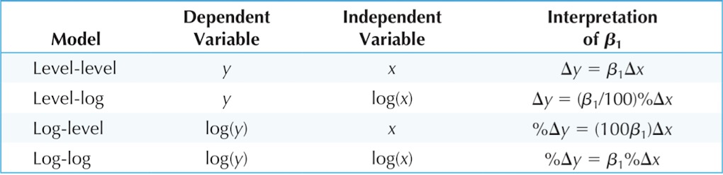
Functional form

• $$log(y)=\beta_0+\beta_1 x+u$$

  • $$\beta_1=\frac{dlog(y)}{dy}=\frac{dy}{y}\cdot\frac{1}{x}$$

• 

Expected Values and Variances of the OLS Estimators

Unbiasedness of OLS

• Unbiasedness means the expectation of the estimator equals the true value.
• 无偏性
• $E(\hat{\beta})=\beta$

假设：SLR（simple linear regression）

1. Linear in Parameters
2. Random Sampling
   • $Cov(u_i,u_j)=0$
3. Sample Variation in the Explanatory Variable
   • 即自变量x的取值不能只有一个点
4. Zero Conditional Mean: $E(u|x) = 0$

在上面四个条件成立时，$\beta_0$ 和 $\beta_1$ 都满足无偏性

• Though the OLS estimator is unbiased, it is still possible that the estimates calculated using the sample is very different from β in the population.

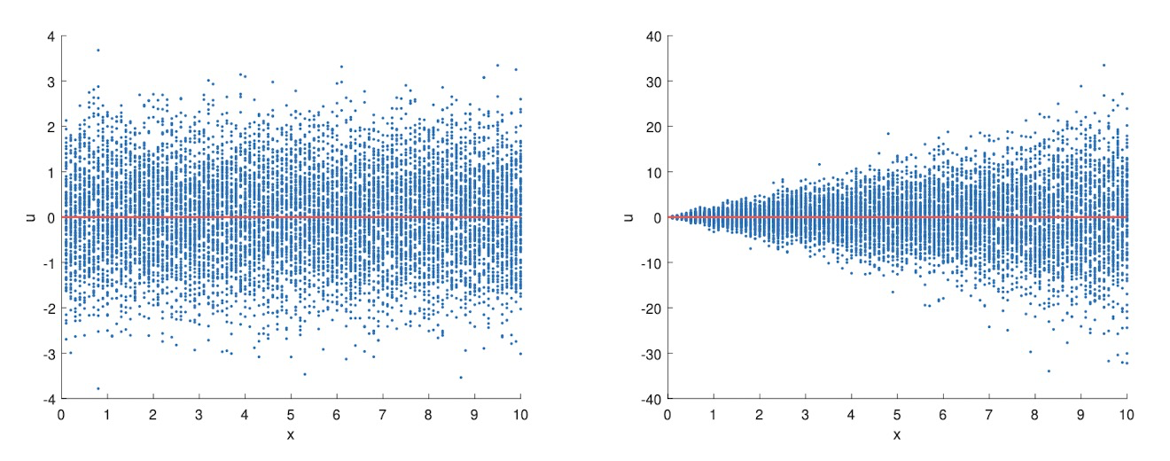
5. Homoskedasticity
   • The error u has the same variance given any value of the explanatory variable.
   • In other words, $Var(u|x)=\sigma^2$
   • 同方差性
   • 

在上面5个条件成立时，可以求方差：

• $$Var(\hat{\beta_1}|x)=\frac{\sigma^2}{\sum_{i=1}^N(x_i-\bar{x})^2}=\frac{\sigma^2}{SST_x}$$
  • 其中 $\sigma$ 是 u 的标准差
  • 当 $\sigma$ 大时$V a r(\hat{\beta}_{1}|x)$ 方差大
  • 当 x 的方差大时 $V a r(\hat{\beta}_{1}|x)$ 小
• $$V a r(\hat{\beta_0}|x)=\frac{\sigma^2\sum_{i=1}^Nx_i^2}{N\sum_{i=1}^N(x_i-\bar{x})^2}$$

估计$\sigma$

• 需要用sample来估计 $\sigma^2$
• $$s^2\equiv\hat{\sigma}^2=\frac{1}{N-2}\sum_{i=1}^N\hat{u}_i^2$$
• 这是无偏估计，其中-2是因为有两个约束条件，少了两个自由度。

Ch3 Multiple Regression Analysis: Estimation

Why we need multiple regression model?

• Descriptive analysis: sometimes we want to estimate the conditional mean of y on multiple variables
• Causal estimation: we know that something other than x may afect y, so we explicitly control them.
• Forecasting: we want to use more variables to better predict y

Estimation and Interpretation

• Population regression model:$$y=\beta_0+\beta_1 x_1+\cdots+\beta_nx_n+u$$
  • zero conditional mean:
    • $$E(u|x_1,\cdots,x_n)=0$$
  • besides, using law of iterated expectation
    • $$E(x_ju)=0\quad E(u)=0$$
• Fitted value: $$\hat{y_i}=\hat{\beta_0}+\hat{\beta_1}x_{i1}+\cdots+\hat{\beta_k}x_{i k}$$
• residual: $$\hat{u_i}= y_{i}-\hat{y_i}$$

Sample analog

population expectations	sample analogue
$E(u)=0$	$\frac{1}{N}\sum \hat{u_i}=0$
$E(x_1u)=0$	$\frac{1}{N}\sum x_{i1}\hat{u_i}=0$
$E(x_ku)=0$	$\frac{1}{N}\sum x_{ik}\hat{u_i}=0$

OLS

• $$H\equiv\sum_{i=1}^n\hat{u_i}^2=\sum(y_i-b_0-b_1x_{i1}-\cdots-b_kx_{i k})^2$$
• 求最小值，得一阶条件：
  • $$\frac{\partial H}{\partial b_0}=-\sum_{i=1}^n2(y_i-\hat{\beta_0}-\hat{\beta_1}x_{i1}-\cdots-\hat{\beta_k}x_{ik})=0$$
  • $${\frac{\partial H}{\partial b_{j}}}=-\sum_{i=1}^{n}2x_{i j}(y_{i}-{\hat{\beta_0}}-{\hat{\beta_1}}x_{i1}-\cdots-{\hat{\beta_k}}x_{i k})=0,\forall j=1,2,…,k.$$
• OLS and sample analogue give the same answer.

Interpretation

• The coeicient of $x_i$ represents holding fixed other factors, the change in y when $x_i$ increases by one unit.

• $$\Delta\hat{y}=\hat{\beta}_1 \Delta x_1+\hat{\beta}_2 \Delta x_2+\cdots+\hat{\beta}_k \Delta x_k$$

• 求 $\hat{\beta_j}$: Frisch-Waugh-Lovell Theorem

  • Regress $x_j$ on other independent variables （including the constant）, obtain the residual $\hat{r_{ij}}$.
  • Regress y on other independent variables （including the constant）, obtain the residual $\hat{r_{iy}}$.
  • Regress $\hat{r_{iy}}$ on $\hat{r_{ij}}$, The resulting slope coefficient is $\hat{\beta_j}$

Goodness of fit

• 和 SLR 相同
• 但随着变量增加 $R^2$ 几乎一定会增大
• 引入 Adjusted R2
  • $$\bar{R}^2=1-\frac{SSR/(N-k-1)}{SST/N-1}=1-(1-R^2)\frac{N-1}{N-k-1}$$
  • N represents the size of the sample, k represents the number of independent variables （excluding the constant）

Expected Values and Variances of the OLS Estimators

假设：MLR（multiple linear regression）

1. Linear in Parameters
2. Random Sampling
   • $Cov(u_i,u_j)=0$
3. No perfect collinearity
   • 不能线性相关
   • 不然无法区别这些线性相关成分
4. Zero Conditional Mean:
   • $E(u|x_1,\cdots,x_k) = 0$

• 在上面四个条件成立时，$\beta_0$ 和 $\beta_1$ 都满足无偏性

5. Homoskedasticity
   • $Var(u|x_1,\cdots,x_k)=\sigma^2$
   • 同方差性

• MLR1-5合成 Gauss-Markov Assumption

• 在Gauss-Markov条件下，方差满足：

  • $$V a r(\hat{\beta_j})=\frac{\sigma^{2}}{SST_j(1-R_j^2)}$$
  • $R_j^2$ is the R-squared from regressing $x_j$ on all other independent variables and including an intercept

• The unbiased estimator of $σ^2$ is:

  • $$\hat{\sigma}^{2}=\frac{1}{N-k-1}\sum_{i=1}^{n}\hat{u}_{i}^{2}.$$
  • 自由度：N-k-1
  • 是无偏估计

BLUE

sdandard deviation	standard error
$sd(\hat{\beta_j})$	$se(\hat{\beta_j})$
$\frac{\sigma}{[SST_j(1-R_j^2)]^{1/2}}$	$\frac{\hat{\sigma}}{[SST_j(1-R_j^2)]^{1/2}}$
$\sigma^2=\text{Var of u}$	$\hat{\sigma}^{2}=\frac{1}{n-k-1}\sum \hat{u}^2$
unknown	estimated using sample

• OLS 是 best linear unbiased estimator, BLUE
  • 满足线性，并且方差最小。

Practical issues

Omitted bias

• 假设有两个自变量，但只对其中一个进行回归，那么得到的$\hat{\beta}$ 与实际值有一个误差。

• $E(\tilde{\beta}_1)=\beta_1+\beta_2\tilde{\delta}_1$

• thus, $Bias(\tilde{\beta_1})=\beta_{2}\tilde{\delta}_{1}$

• 	$Corr(x_1,x_2)>0$	$Corr(x_1,x_2)<0$
  $\beta_2>0$	Positive Bias	Negative Bias
  $\beta_2<0$	Negative Bias	Positive Bias

• 影响无偏性

including irrelavent

• 不影响无偏性，但方差会变大

Multicollinearity

• high （but not perfect） correlation between two or more independent variables
• 不影响无偏性，但方差会变大

Ch4 Multiple Regression Analysis: Inference

Classical Linear Regression Model

The Distribution of $\hat{β_j}$

• 为了得到分布，在Gauss-Markov条件上还要加上一条：

• MLR6: Normality

  • $$u\sim N(0,\sigma^2)$$

• Assumptions MLR.1 through MLR.6 are called the classical linear model CLM assumptions.

• summarize the population assumptions of the CLM is

  • $$y|{\bf x}\ \sim\ No r m a l(\beta_{0}\ +\beta_{1}x_{1}+\ldots+\beta_{k}x_{k},\sigma^{2})$$

• 在CLM条件下，$\beta$ 服从正态分布

  • $$\frac{\hat{\beta}_j-\beta_j}{sd(\hat{\beta}_j)}\sim Normal(0,1)$$

• 但由于实际中标准差不知道，需要用标准误来算。

  • $$\frac{\hat{\beta_j}-\beta_j}{s e(\hat{\beta_j})}\sim t_{N-k-1}= t_{d f},$$
  • 服从t分布，N-k-1是自由度，N是多少个样本，k是回归里面有多少个x

t检验

• 检验某个系数是否为0

Null hypothesis

• Let $H_0$ be the null hypothesis that we want to test. Let $H_1$ be the alternative hypothesis.
• We reject the null hypothesis when the test statistic falls in the rejection region.

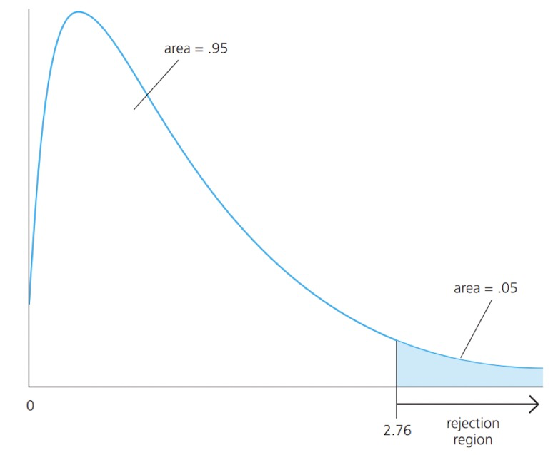
rejection region

• type 1 error:
  • significance level = α = $Pr(\text{rejecting }H_0|H_0\text{ is true})$
• type 2 error:
  • $Pr(\text{not rejecting }H_0|H_1\text{ is true})$
• 我们的想法是先固定一个significance level，确定对type 1 error 的容忍度，然后再最小化 type 2 error

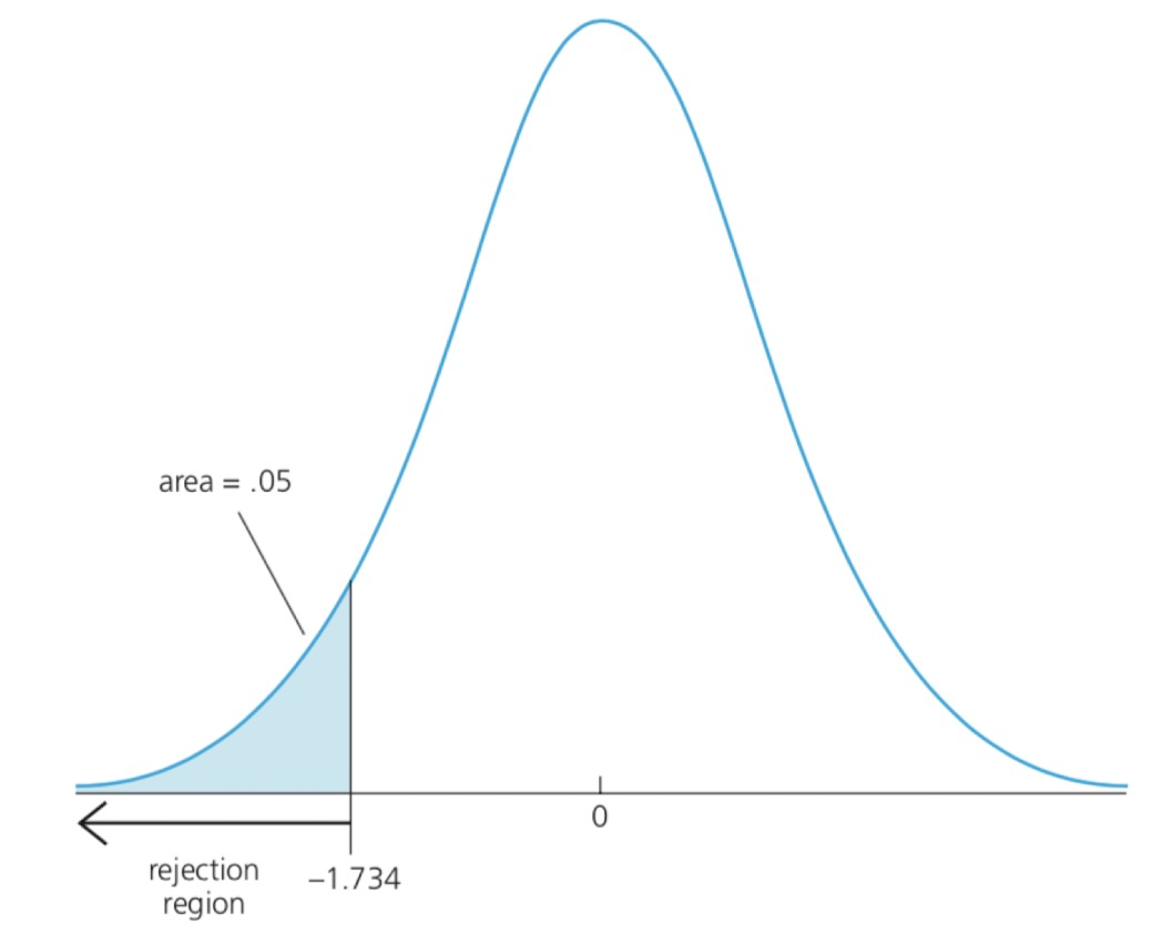
Testing Against One-Sided Alternatives

• Suppose we are interested in testing
  $$
  \begin{array}{ll}
  H_0: & \beta_j=0 . \\
  H_1: & \beta_j>0 .
  \end{array}
  $$
• Consider a test statistic:$$\frac{\hat{\beta}_j-\beta_j}{\operatorname{se(}(\hat{\beta}_j)}$$
• When $H_0$ is true, the test statistic is: $$\frac{\hat{\beta_j}}{s e(\hat{\beta_j})} \sim t_{N-k-1}=t_{df}$$

1. It depends on the data.
2. We know its distribution under $H_0$.

• 令 $$t_{\hat{\beta}_j} \equiv \frac{\hat{\beta}_j}{s e(\hat{\beta}_j)}$$
• We often call $t_{\hat{\beta}_j}$ t-statistic or t-ratio of $\hat{\beta}_j$.
• $t_{\hat{\beta}_j}$ has the same sign as $\hat{\beta}_j$, because $\operatorname{se}(\hat{\beta}_j)>0$.

• 直觉上, 当 $t_\hat{\beta_j}$ 足够大的时候拒绝 $H_0$ : $t_\hat{\beta_i}$ 越大, $H_0$ 是真的可能性越低, $H_1$ 是真的可能性越高。

• 多大算足够大？
  • Fix a significance level of $5 %$. The critical value, $c$ is the 95 th percentile when $H_0$ is true. It means when $H_0$ is true, the probability of getting a value as large as $c$ is $5 %$.
  • Rejection rule:$t_{\hat{\beta}_j}>c$
• Rejecting $H_0$ when $t_{\hat{\beta}_j}>c$ means the probability of making a type I error, that is, the probability of rejecting $H_0$ when $H_0$ is true, is $5 %$.
• 

The idea of test

1. Fix a significance level $\alpha$. That is, decide our level of “tolerence” for the type I error.
2. Find the critical value associated with $\alpha$. For $H_1: \beta_j>0$, this means finding the $(1-\alpha)$-th percentile of the $\mathrm{t}$ distribution with $d f=N-k-1$.
3. Reject $H_0$ if $t_{\hat{\beta}_j}>c$

• 通常第一类错误和第二类错误是不能同时缩小的。需要取舍。

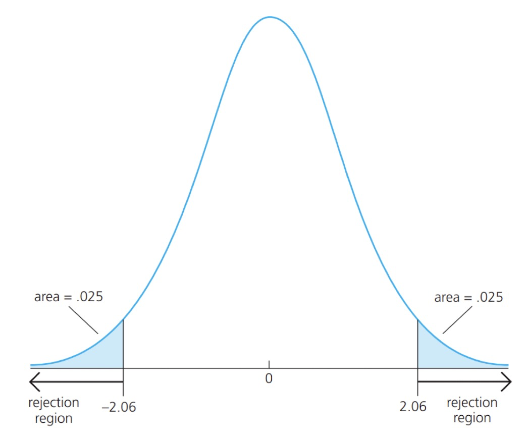
Two-sided Alternatives

• We want to test:$$\begin{array}{ll}H_0: & \beta_j=0 . \\ H_1: & \beta_j \neq 0 .
  \end{array}$$

• This is the relevant alternative when the sign of $\beta_j$ is not well determined by theory.

• Even when we know whether $\beta_j$ is positive or negative under the alternative, a two-sided test is often prudent.

• 求法：

  1. Fix a significance level $\alpha$. That is, decide our level of “tolerence” for the type I error.
  2. Find the critical value associated with $\alpha$. For $H_1: \beta_j \neq 0$, this means finding the $(1-\alpha / 2)$-th percentile of the $\mathrm{t}$ distribution with $d f=N-k-1$.
  3. Reject $H_0$ if$$|t_{\hat{\beta}_j}|>c .$$

• 

• 没有说明的话通常是双边的

• If $H_0$ is rejected in favor of $H_1: \quad \beta_j \neq 0$ at the $5 %$ level, we usually say that “ $x_j$ is statistically significant, or statistically different from zero, at the $5 %$ level.”

• If $H_0$ is not rejected, we say that “ $x_j$ is statistically insignificant at the $5 %$ level.”

Other Hypothesis

• If the null is stated as:
  $$
  H_0: \beta_j=a_j
  $$
  Then the t-statistic is$$\frac{\hat{\beta_j}-a_j}{\operatorname{se}(\hat{\beta_j})} \sim t_{N-k-1}$$
  We can use the general t statistic to test against one-sided or two-sided alternatives.

p-Values for t Tests

• Given the observed value of the t statistic, what is the smallest significance level at which the null hypothesis would be rejected?
• We call this “smallest signiicance level” p-value.
• p-value represents the probability of observing a value as extreme as $t_{\hat{\beta}_j}$ under the $H_0$
• $$
  \begin{array}{ll}
  H_0: & \beta_j=0 . \\
  H_1: & \beta_j \neq 0 .
  \end{array}
  $$
  • The p-value in this case is$$P(|T|>|t|),$$
  • where we let $T$ denote a $\mathrm{t}$ distributed random variable with $N-k-1$ degrees of freedom and let $t$ denote the numerical value of the test statistic.

• The p-value nicely summarizes the strength or weakness of the empirical evidence against the null hypothesis.
• The p-value is the probability of observing a $t$ statistic as extreme as we did if the null hypothesis is true.
• Signiicance level and critical value一一对应

Economic versus Statistical Signiicance

• The statistical significance of a variable $x_j$ is determined entirely by the size of $t_{\hat{\beta}_j}$, whereas the economic significance or practical significance of a variable is related to the size (and sign) of $\hat{\beta}_j$.

• We often care about both statistical significance and economic significance.

Confidence interval

• We can construct a confidence level depending on $\alpha$. We call it a $(1-\alpha)$ confidence interval:$$[\hat{\beta}_j-c \cdot \operatorname{se}(\hat{\beta}_j), \hat{\beta}_j+c \cdot \operatorname{se}(\hat{\beta}_j)]$$
• The critical value $c$ is the $(1-\alpha / 2)$ percentile in a $\mathrm{t}$ distribution with $d f=N-k-1$.
• The meaning of a 95% conidence interval: if we sample repeatedly many times, then the true $β_j$ will appear in 95% of the confidence intervals.
• 对于很多次取样来说的可能性，但对于某一次特定的取样不能确定是否一定在置信区间里面。

三种方法一样：

1. Fix a significance level $\alpha$, calculate the critical value $c$, and then reject $H_0$ if $|t_{\hat{\beta}_j}|>c$.
2. Fix a significance level $\alpha$, calculate the $\mathrm{p}$-value, reject $H_0$ if $p<\alpha$.
3. reject if 0 is not in the confidence level.

Testing Multiple Linear Restrictions: The F Test

• $$y=\beta_0+\beta_1 x_1+\beta_2 x_2+\beta_3 x_3+u$$We want to test$$H_0: \quad \beta_1=0 \text { and } \beta_2=0$$$$H_1: H_0\text{ is not true.}$$
• Method:
  • Consider the restricted model when $H_0$ is true$$y=\gamma_0+\gamma_3 x_3+u$$
  • If $H_0$ is true, the two models are the same. That means when we include $x_1$ and $x_2$ into the model, the sum of squared residuals should not change much.
  • However, if $H_0$ is false that means that at least one of $\beta_1, \beta_2$ is nonzero and the sum of squared residuals should fall when we include these new variables
  • 看SSR是否相等

• F-test
  • $$F \equiv \frac{(S S R_r-S S R_{u r}) / q}{S S R_{u r} /(N-k-1)}= \frac{(R_{u r}^2-R_r^2) / q}{(1-R_{u r}^2) /(N-k-1)}$$
  • $q$ is the number of linear restrictions, which is the difference in degrees of freedom in the restricted model versus the unrestricted model.
  • $S S R_r$ is the sum of squared residuals from the restricted model and $S S R_{u r}$ is the sum of squared residuals from the unrestricted model.
  • Since $S S R_r$ can be no smaller than $S S R_{u r}$, the $\mathrm{F}$ statistic is always nonnegative.
  • We can show that the sampling distribution of the F-stat: $F \sim F_{q, N-k-1}$. We call this an $\mathrm{F}$ distribution with $q$ degrees of freedom in the numerator and $N-k-1$ degrees of freedom in the denominator.
  • 
• t分布的平方就是F分布，因此单变量也可以用F分布。
• In the $\mathrm{F}$ testing context, the $\mathrm{p}$-value is defined as$$P(\mathcal{F}>F) $$where $\mathcal{F}$ denote an $\mathrm{F}$ random variable with $(q, N-k-1)$ degrees of freedom, and $\mathrm{F}$ is the actual value of the test statistic.
• p-value is the probability of observing a value of $\mathrm{F}$ at least as large as we did, given that the null hypothesis is true.
  • $\rightarrow$ Reject $H_0$ if $p<\alpha$

• 通常情况下使用SSR形式的F检验比较好，因为有时候restricted的形式与unrestricted不同，不能直接用R2来计算。

Testing Multiple Linear Restrictions: The LM statistic

• Lagrange multiplier （LM） statistic
• The LM statistic can be used in testing multiple exclusion restrictions （as in an $F$ test） under large sample.
• 对于模型$$y=\beta_0+\beta_1 x_1+\ldots+\beta_k x_k+u$$We want to test whether the last $q$ of these variables all have zero population parameters:$$H_0: \beta_{k-q+1}=\beta_{k-q+2}=\ldots=\beta_k=0$$

• $L M$ statistic
• First estimate the restricted model:$$y=\tilde{\beta_0}+\tilde{\beta_1} x_1+\cdots+\tilde{\beta_{k-q}} x_{k-q}+\tilde{u}$$If the coefficients of the excluded independent variables $x_{k-q+1}$ to $x_k$ are truly zero in the population model, then they should be uncorrelated to $\tilde{u}$.
• So regress $\tilde{u}$ on all $x$$$\tilde{u} \sim x_1, x_2, \ldots, x_k$$Let $R_u^2$ denote the R-squared of this regression. The smaller the $R_u^2$, the more likely $H_0$ is true. So a large $R_u^2$ provides evidence against $H_0$.
• $L M=N \cdot R_u^2$. We can show that $L M$ follows chi-square distribution with $q$ degrees of freedom: $\mathcal{X}_q^2$.
  • Reject $H_0$ if $L M>$ critical value $(p<$ significance level)
  • 
• 在大样本时，LM和F检验结果很相似

Ch5 Multiple Regression Analysis: OLS Asymptotics

Asymptotic Properties

• Finite sample properties: properties hold for any sample of data.
• Examples
  • Unbiasedness of OLS
  • OLS is BLUE
  • Sampling distribution of the OLS estimators
• Asymptotic properties or large sample properties: not defined for a particular sample size; rather, they are defined as the sample size grows without bound.
  • 渐近性质

Consistency

• 一致性
• Let $W_N$ be an estimator of $\theta$ based on a sample $Y_1, Y_2, \ldots, Y_N$ of size $N$. Then, $W_N$ is a consistent estimator of $\theta$ if for every $\epsilon>0$$$P(|W_N-\theta|>\epsilon) \rightarrow 0 \text { as } N \rightarrow \infty .$$
• We also say consistency means:$$\operatorname{plim}(W_N)=\theta$$
  • Intuitively, consistency means when the sample size becomes larger, the estimator gets closer and closer to the true value.
• 一致性和无偏性没有必然联系

Consistency of OLS

• Under Assumptions MLR.1 through MLR.4, the OLS estimator $\hat{\beta}_j$ is consistent for $\beta_j$, for all $j=0,1, \ldots, k$.

• When the sample size is larger, the OLS estimator is centered around the true parameter closer and closer.

Central Limit Theorem

• Use the notation$$\hat{\theta}_N \stackrel{a}{\sim} N(0, \sigma^2)$$to mean that as the sample size $N$ gets larger, $\hat{\theta}_N$ is approximately normally distributed with mean 0 and variance $\sigma^2$.
• Central Limit Theorem
  • Let ${Y_1, Y_2, \ldots, Y_N}$ be a random sample with mean $\mu$ and variance $\sigma^2$. Then,$$Z_N=\frac{\bar{Y}_N-\mu}{\sigma / \sqrt{N}} \stackrel{a}{\sim} N(0,1)$$
  • Intuitively, it means when the sample size gets larger, the distribution of the sample average is closer to a normal distribution.
  • 不管Y的分布如何，当样本量足够大，都会趋向于正态分布

Asymptotic Normality of OLS

• Under the Gauss-Markov Assumptions MLR.1 through MLR. 5 , for each $j=0,1, \ldots, k$
• $$\begin{aligned}
  & \frac{\hat{\beta}_j-\beta_j}{s d(\hat{\beta}_j)} \stackrel{a}{\sim} \operatorname{Normal}(0,1) . \\
  & \frac{\hat{\beta}_j-\beta_j}{\operatorname{se}(\hat{\beta}_j)} \stackrel{a}{\sim} \operatorname{Normal}(0,1) .
  \end{aligned}$$
• OLS estimators are approximately normally distributed in large enough sample sizes.
• 这个定理说明当样本量足够大的时候，不需要u的正态分布假定。

Summary

• Under MLR.1-MLR.4, OLS estimators are consistent.
• Under MLR.1-MLR.5, OLS estimators have an asymptotic normal distribution.

Ch6 Multiple Regression Analysis: Further Issues

Efects of Data Scaling on OLS Statistics

changing unit of measurement

• Consider the simple regression model:$$y=\beta_0+\beta_1 x+u$$
• Now suppose $y^*=w_1 y$ and $x^*=w_2 x$, Then for this model:$$y^*=\beta_0^*+\beta_1^* x^*+u$$
• $\hat{\beta}_0^*$ and $\hat{\beta}_0$, and $\hat{\beta}_1^*$ and $\hat{\beta}_1$ 的关系是？
  • $$\hat{\beta}_0^*=w_1 \hat{\beta}_0, \quad \hat{\beta}_1^*=\frac{w_1}{w_2} \hat{\beta}_1$$
  • $$\operatorname{se}(\hat{\beta}_0^*) =w_1 \operatorname{se}(\hat{\beta}_0), \quad\operatorname{se}(\hat{\beta}_1^*) =\frac{w_1}{w_2}\operatorname{se}(\hat{\beta}_1)$$
  • $$t_\hat{\beta_0}^*=t_\hat{\beta_0} \quad t_\hat{\beta_1}^* =t_\hat{\beta_1}$$
  • $$R^{2*}=R^2$$
  • the statistical signiicance does not change.

Unit Change in Logarithmic Form

• 只影响截距，不影响系数

Beta Coefficients

• Sometimes, it’s useful to obtain regression results when all variables are standardized: subtracting off its mean and dividing by its standard deviation.
• $$
  \begin{aligned}
  y_i & =\hat{\beta_0}+\hat{\beta_1} x_{i 1}+\cdots+\hat{\beta_k} x_{i k}+\hat{u_i} . \\
  (y_i-\bar{y}) / \hat{\sigma_y} & =(\hat{\sigma_1} / \hat{\sigma_y}) \hat{\beta_1}[(x_{i 1}-\bar{x_1}) / \hat{\sigma_1}]+\cdots \\
  & +(\hat{\sigma_k} / \hat{\sigma_y}) \hat{\beta_k}[(x_{i k}-\bar{x_k}) / \hat{\sigma_k}]+(\hat{u_i} / \hat{\sigma_y}) \\
  z_y & =\hat{b_1} z_1+\cdots+\hat{b_k} z_k+\text { error }
  \end{aligned}
  $$
• where $z_y$ denotes the z-score of $y$. The new coefficients are$$\hat{b}_j=(\hat{\sigma}_j / \hat{\sigma}_y) \hat{\beta}_j$$
• If $x_1$ increases by one standard deviation, then $\hat{y}$ changes by $\hat{b}_1$ standard deviation.
• 归一化了

More on Functional Form

• 对于log形式 $$z=log(y)=\beta_0+\beta_1 x+u$$
  • 当x变化$\Delta$ 时，$$\%\Delta E(y|x)=100[exp(\beta_1\Delta)-1]$$
  • 当 $\Delta$ 趋近0时，$$\%\Delta E(y|x)\approx 100\beta_1\Delta$$
• 对于x取值小于0的，可以使用 inverse hyperbolic sine: $$IRS(x)=arcsinh(x)=log(x+\sqrt{x^2+1})$$
• 当x对y的影响是非线性的，可以考虑二次方。

More on Goodness of Fit

• 在Ch4中通过F检验来判断是否可以restrict模型，那么对于non-nested model怎么办呢？
• 例如： $$\begin{aligned}
  & y=\beta_0+\beta_1 x_1+\beta_2 x_2+u \\
  & y=\gamma_0+\gamma_1 x_4+e
  \end{aligned}$$
• 这时候需要用 Adjusted R-square
  • 选择 $\bar{R}^2$ 最高的

Prediction Analysis

confidence interval for E(y|x)

• Suppose we have estimated the equation$$\hat{y}=\hat{\beta}_0+\hat{\beta}_1 x_1+\hat{\beta}_2 x_2+\ldots+\hat{\beta}_k x_k$$Let $c_1, c_2, \ldots, c_k$ denote particular values for each of the $k$ independent variables.
• The parameter we would like to estimate is$(\theta)=E(y \mid x_1=c_1, \ldots, x_k=c_k)=\beta_0+\beta_1 c_1+\beta_2 c_2+\ldots+\beta_k c_k$
• The estimator of $\theta$ is$$\hat{\theta}=\hat{\beta}_0+\hat{\beta}_1 c_1+\hat{\beta}_2 c_2+\ldots+\hat{\beta}_k c_k$$
• $$y=\theta+\beta_1(x_1-c_1)+\beta_2(x_2-c_2)+\ldots+\beta_k(x_k-c_k)+u$$

• So we can regress $y_i$ on $(x_{i 1}-c_1), \ldots,(x_{i k}-c_k)$. The standard error and confidence interval of the intercept of this new regression is what we need.

Prediction Interval

• $$y=E(y \mid x_1, \ldots, x_k)+u$$
• The previous method form a confidence interval for $E(y \mid x_1, \ldots, x_k)$.

• Sometimes we are interested in forming the confidence interval for an unknown outcome on $y$.
• We need to account for the variation in $u$.

• Let $x_1^0, \ldots, x_k^0$ be the new vales of the independent variables, which we assume we observe. Let $u^0$ be the unobserved error.
  $$
  y^0=\beta_0+\beta_1 x_1^0+\ldots+\beta_k x_k^0+u^0 .
  $$
• Our best prediction of $y^0$ is estimated from the OLS regression line
  $$
  \hat{y}^0=\hat{\beta}_0+\hat{\beta}_1 x_1^0+\ldots+\hat{\beta}_k x_k^0
  $$
• The prediction error in using $\hat{y}^0$ to predict $y^0$ is
• Note $E(\hat{y}^0)=y^0$, because the $\hat{\beta}_j$ are unbiased. Because $u^0$ has zero mean, $E\left(\hat{e}^0\right)=0$.
• Note that $u^0$ is uncorrelated with each $\hat{\beta}_j$, because $u^0$ is uncorrelated with the errors in the sample used to obtain the $\hat{\beta}_j$.

• Therefore, the variance of the prediction error (conditional on all in-sample values of the independent variables) is:
  $$
  \operatorname{Var}(\hat{e}^0)=\operatorname{Var}(\hat{y}^0)+\operatorname{Var}(u^0)=\operatorname{Var}(\hat{y}^0)+\sigma^2 .
  $$

• The standard error of $\hat{e}^0$ is:$$se(\hat{e}^0)={[se(\hat{y}^0)]^2+\hat{\sigma}^2}^{1 / 2}$$
• The prediction interval for $y^0$ is
  $$
  \sqrt{\hat{y}^0 \pm c \cdot s e\left(\hat{e}^0\right)}
  $$

Ch7 Multiple Regression Analysis with Qualitative Information

A Single Dummy Independent Variable

• We often capture binary information by defining binary variable or a zero-one variable.$$\text { female }= \begin{cases}0, & \text { if the individual is man } \\ 1, & \text { if the individual is woman }\end{cases}$$

• zero-one leads to natural interpretations of the regression parameters

• 假设 $$\text { wage }=\beta_0+\delta_0 \text { female }+u$$

• If we estimate the model using OLS$$\begin{aligned}
  & \hat{\beta_0}=\overline{w a g e_{m e n}} \\
  & \hat{\delta_0}=\overline{w a g e_{women}}-\overline{w a g e_{m e n}}\end{aligned}$$

• If we regress $y$ on a dummy variable $x$, then the OLS estimate of the intercept represents the sample average of $y$ when $x=0$, the OLS estimate of the slope coefficient represents the difference between the sample average of $y$ when $x=1$ and $x=0$.

• 当增加变量时，例如 $$w a g e=\beta_0+\delta_0 \text { female }+\beta_1 e d u c+u$$

• $δ_0$ is the difference in hourly wage between women and men, given the same amount of education.

线性相关

• $wage=\beta_0 + \beta_1female+u$ 是可以的
  • 选定了 male 作为 baseline group
• $wage=\beta_0 male + \beta_1female+u$ 是可以的
• $wage=\beta_0+\beta_1 male + \beta_2female+u$ 是不行的

Without intercept

• $wage=\beta_0 male + \beta_1female+u$ 没有截距，在解释和计算检验的时候不方便，并且 $R^2$ 可能是负的。
• In general, if there is no intercept in the regression model, the $R^2$ could be negative.
• To address the issue, some researchers use the uncentered R-squared when there is no intercept in the model$$R_0^2=1-\frac{S S R}{S S T_0},$$where $S S T_0=\sum_{i=1}^N y_i^2$.

Using Dummy Variables for Multiple Categories

• 多个组别的时候，两种选择

• 第一种，k-1个独立的变量：

  • $$\text { wage }=\beta_0+\beta_1 \text { marrmale }+\beta_2 \text { marrfemale }+\beta_3 \text { singfem }+u \text {. }$$

• 第二种，乘积项：

  • $$\text { wage }=\beta_0+\beta_1 \text { female }+\beta_2 \text { married }+\beta_3 \text { female } \cdot \text { married }+u$$

• 注意如果一个变量只能在几个离散值之间选择，最好把每个值的情况独立成一个哑元，否则相当于暗示了斜率变化是线性的。

  • 例如CR可以取0，1，2，3，4
  • $$MBR=\beta_0+\beta_1 C R+\text { other factors }+u \text {. }$$
  • $$MBR=\beta_0+\delta_1 C R 1+\delta_2 C R 2+\delta_3 C R 3+\delta_4 C R 4+\text{other factors}+u$$
  • 第二种模型更好。

Interactions Involving Dummy Variables

• 在 $wage=\beta_0+\beta_1female+\beta_2educ+u$ 中我们假定了 educ 对于男女的影响是相同的。
• 为了区别，需要添加一个乘积项：$$E(\text { wage } \mid \text { female }, \text { educ })=\beta_0+\delta_0 \text { female }+\beta_1 \text { educ }+\delta_1 \text { female } \cdot \text { educ. }$$

Testing for Differences in Regression Functions across Groups

• $$\text { wage }=\beta_0+\beta_1 \text { educ }+\beta_2 \text { exper }+\beta_3 \text { tenure }+u$$

• We want to test whether all the coefficients are the same for men and women.
• We can include interactive terms for all variables:$$
  \begin{aligned}
  \text { wage }= & \beta_0+\delta_0 \text { female }+\beta_1 \text { educ }+\delta_1 \text { educ } \cdot \text { female }+ \\
  & \beta_2 \text { exper }+\delta_2 \text { exper } \cdot \text { female }+ \\
  & \beta_3 \text { tenure }+\delta_3 \text { tenure } \cdot \text { female }+u .
  \end{aligned}$$

• The null hypothesis:$$H_0: \delta_0=0, \delta_1=0, \delta_2=0, \delta_3=0$$We can use F test to test the hypothesis: estiamte the unrestricted and restricted model, and then calculate the F-stat.

Chow statistic

• 对于只有一个二元变量和很多其他连续变量的回归，我们想判断其他所有的变量是否关于两组完全相同
• We can show that the sum of squared residuals from the unrestricted model can be obtained from two separate regressions, one for each group: $S S R_{u r}=S S R_1+S S R_2$
• The F-statstic:$$F=\frac{S S R_p-(S S R_1+S S R_2)}{S S R_1+S S R_2} \cdot \frac{N-2(k+1)}{k+1}$$$S S R_p$ : SSR from pooling the groups and estimating a single equation.
• This is also called a Chow statistic.
• Note: use the Chow test if
  • the model satisfies homoskedasticity
  • we want to test no differences at all between the groups

Program Evaluation

• 在社会学实验中控制变量法

Ch8 Heteroskedasticity

Consequence of Heteroskedasticity for OLS

• Heteroskedasticity does not cause bias or inconsistency in the OLS estimators
  • 对于一致性和无偏性无影响
• The interpretation of our goodness-of-fit measures is also unaffected by the presence of heteroskedasticity.
  • 对于goodness of fit 无影响
  • $R^2$ and adj- $R^2$ are different ways of estimating the population R-squared, $1-\sigma_u^2 / \sigma_y^2$.
  • both variances in the population $R^2$ are unconditional variances
  • SSR/ $N$ consistently estimates $\sigma_u^2$, and $S S T / N$ consistently estimates $\sigma_y^2$, whether or $\operatorname{not} \operatorname{Var}(u \mid x)$ is constant

• With heteroskedasticity, $\operatorname{Var}\left(\hat{\beta}_j\right)$ is biased.
  • 对于方差有影响
  • 标准差，t数据，置信区间都不再可靠
  • 大样本也不能解决
  • OLS is no longer BLUE.

Heteroskedasticity-Robust Inference after OLS Estimation

• Consider the simple linear regression model:$$y_i=\beta_0+\beta_1 x_i+u_i$$Assume SLR.1-SLR.4 are satisfied, and there exists heteroskedasticity:$$\operatorname{Var}(u \mid x_i)=\sigma_i^2$$$\operatorname{Var}(u)$ takes on different values when $x$ varies

• We don’t know the exact functional form of $\sigma_i^2$, it can be any function of $x$

Estimating $\operatorname{Var}\left(\hat{\beta}_j\right)$ under Heteroskedasticity

• One valid estimator （White,1980）:$$\widehat{\operatorname{Var}}(\hat{\beta_1})=\frac{\sum_{i=1}^N(x_i-\bar{x})^2 \hat{u_i}^2}{[\sum_{i=1}^N(x_i-\bar{x})^2]^2} \equiv \frac{\sum_{i=1}^N(x_i-\bar{x})^2 \hat{u_i}^2}{SST_x^2}$$where $$SST_x=\sum_{i=1}^N(x_i-\bar{x})^2$$.
• For multiple regression model:$$\begin{gathered}y_i=\beta_0+\beta_1 x_{i 1}+\beta_2 x_{i 2}+\ldots+\beta_k x_{i k}+u_i . \\ \operatorname{Var}(\hat{\beta_j})=\frac{\sum_{i=1}^N \hat{r_{ij}}^2 \sigma_i^2}{[\sum_{i=1}^N \hat{r_{ij}}^2]^2} \equiv \frac{\sum_{i=1}^N \hat{r_{ij}}^2 \sigma_i^2}{SSR_j^2}\end{gathered}$$The estimator:$$\widehat{\operatorname{Var}}(\hat{\beta_j})=\frac{\sum_{i=1}^N \hat{r_{ij}}^2 \hat{u_i}^2}{[\sum_{i=1}^N \hat{r_{ij}}^2]^2}=\frac{\sum_{i=1}^N \hat{r_{ij}}^2 \hat{u_i}^2}{SSR_j^2}$$
  • $\hat{r_{ij}}$ is the residual from regressing $x_j$ on all other independent variables
  • $S S R_j$ is the sum of residual squared of this regression
  • The square root of $\widehat{\operatorname{Var}}\left(\hat{\beta}_j\right)$ is called the heteroskedasticity-robust standard error, or simply, robust standard errors.
• Robust-standard error 是一致的

Compare the variance formula

• Under homoskedasticity, $\operatorname{Var}(\hat{\beta_1})$ is simplified as$$\operatorname{Var}(\hat{\beta_j})=\frac{\sum_{i=1}^N \hat{r_{ij}}^2 \sigma_i^2}{SSR_j^2}=\frac{\sigma^2}{SSR_j}$$
• Under heteroskedasticity,$$\operatorname{Var}(\hat{\beta_j})=\frac{\sum_{i=1}^N r_{i j}^2 \sigma_i^2}{SSR_j^2}=\frac{1}{SSR_j} \sum_{i=1}^N \frac{\hat{r_{ij}}^2}{SSR_j} \sigma_i^2=\frac{1}{SSR_j} \sum_{i=1}^N w_{ij} \sigma_i^2$$where $w_{ij}=\frac{\hat{\tau_{ij}}^2}{S S R_j}$. We know that $w_{ij}>0$ and $\sum_{i=1}^N w_{ij}=1$.
• 即，进行了加权平均。
• Robust standard errors can be either larger or smaller than the usual standard errors.

More on RSE

• 在有些情况下，特别是异方差性不强的情况下，robust-standard-error的表现不如传统的standard-error
  • 小样本时rse存在误差
  • rse的样本方差更大
• 在实践中通常在大样本时报告rse，在小样本时都报告。

Weighted Least Squares Estimation

Generalized Least Squares （GLS）

• Assume MLR.1-MLR.4 are satisfied:$$y_i=\beta_0+\beta_1 x_{i 1}+\ldots+\beta_k x_{i k}+u_i$$
• Assume that the variance of $u$ takes the following form:$$\operatorname{Var}(u \mid x_1, \ldots, x_k)=\sigma^2 h(x_1, \ldots, x_k)$$
• We write $\sigma_i^2=\sigma^2 h\left(x_{i 1}, \ldots, x_{i k}\right)=\sigma^2 h_i$.

• Consider an alternative regression model:$$\frac{y_i}{\sqrt{h_i}}=\beta_0 \frac{1}{\sqrt{h_i}}+\beta_1 \frac{x_{i 1}}{\sqrt{h_i}}+\ldots+\beta_k \frac{x_{i k}}{\sqrt{h_i}}+\frac{u_i}{\sqrt{h_i}}$$

• Let $\mathbf{x}$ denote all the explanatory variables. Conditional on $\mathbf{x}, E\left(u_i / \sqrt{h_i} \mid \mathbf{x}\right)=E\left(u_i \mid \mathbf{x}\right) / \sqrt{h_i}=0$.
• $\operatorname{Var}\left(u_i / \sqrt{h_i} \mid \mathbf{x}\right)=\sigma^2$, satisfying homoskedasticity.
• Denote the OLS estimator after the transformation as ${\beta_j^*}$
• We can prove that ${\beta_j^*}$ minimizes$$\sum_{i=1}^N(y_i-b_0-b_1 x_{i 1}-\cdots-b_k x_{i k})^2 / h_i$$
• Weighted least squares estimator（WLS）:
  • the weight for each $\hat{u}_i$ is $1 / h_i$. We give less weight for observations with higher variance. Intuitively, they provide less information.
• ${\beta_j^*}$ is still one estimator for the original model, and have the same interpretation
• Because ${\beta_j^*}$ satisfies MLR.1-MLR.5, so it is BLUE under heteroskedasticity with the form $\sigma_i^2=\sigma^2 h_i$
• ${\beta_j^*}$ is also called generalized least squares estimators （GLS）

Feasible Generalized Least Squares （FGLS）

• 实际中需要估计 $h_i$

• Assume $h_i$ takes the following form:$$\begin{aligned}\operatorname{Var}(u \mid x) & =\sigma^2 \exp \left(\delta_0+\delta_1 x_1+\ldots+\delta x_k\right) \\ u^2 & =\sigma^2 \exp \left(\delta_0+\delta_1 x_1+\ldots+\delta x_k\right) v,\end{aligned}$$where $v$ has a mean of one.
• We take $\exp (\cdot)$ to guarantee that $\operatorname{Var}(u)>0$
• Equivalently,
  $$
  \log \left(u^2\right)=\alpha+\delta_1 x_1+\ldots+\delta x_k+e .
  $$

• As usual, we replace the unobserved $u$ with the OLS residuals $\hat{u}$, and estimate $\log \left(\hat{u}^2\right) \sim 1, x_1, \ldots x_k$, calculate the fitted value $\hat{g}_i$. Then $\hat{h}_i=\exp \left(\hat{g}_i\right)$.

Procedure

1. Run the regression of $y$ on $1, x_1, \ldots, x_k$, get the residual $\hat{u}_i$
2. Calculate $\log \left(\hat{u}_i^2\right)$
3. Estimate $\log \left(\hat{u}_i^2\right) \sim 1, x_1, \ldots x_k$, get the fitted value $\hat{g}_i$
4. Compute $\hat{h}_i=\exp \left(\hat{g}_i\right)$
5. Use $1 / \hat{h}_i$ as weights, estimate $y \sim 1, x_1, \ldots, x_k$ using WLS.

FGLS is consistent, and has smaller asymptotic variance than OLS.

WLS or RSE

• There is no guarantee that WLS is more efficient than OLS.

• It is alwasy advised to report robust standard errors with WLS.

• two solutions for heteroskedasticity:
  • Use OLS to estiamte the model, calculate the robust standard errors （or use the max of the conventional s.e. and robust s.e.）
  • Use FGLS to estimate the model, report conventional s.e. or robust s.e.
• In practice, the first method is preferred in most cases

Testing for Heteroskedasticity

Breusch-Pagan Test for Heteroskedasticity

• We want to know in model $y=\beta_0+\beta_1 x_1+. .+\beta_k x_k+u$, whether $u^2$ is correlated with $x$
• Estimate $y=\beta_0+\beta_1 x_1+. .+\beta_k x_k+u$, get the residual $\hat{u}$
• Estimate the following model and get $R_{\hat{u}^2}^2$ :$$\hat{u}_i^2=\delta_0+\delta_1 x_1+\ldots+\delta_k x_k+v$$
• We test $H_0: \delta_1=\ldots=\delta_k=0$
• Calculate the $L M$ statistic: $N \cdot R_{\hat{u}^2}^2$; or calculate the $F$ $\operatorname{statistic}\left[R_{\hat{u}^2}^2 / k\right] /\left[\left(1-R_{\hat{u}^2}^2\right) /(N-k-1)\right]$.
• Reject homoskedasticity if
  • test statistic $>$ critical value
  • $p<$ significance level

The White Test for Heteroskedasticity

• OLS standard errors are asymptotically valid if MLR.1-MLR.5 holds.
• It turns out that the homoskedasticity assumption can be replaced with the weaker assumption that the squared error, $u^2$, is uncorrelated with all the independent variables $\left(x_j\right)$, the squares of the independent variables $\left(x_j^2\right)$, and all the cross products $\left(x_j x_h, \forall j \neq h\right)$.

• When the model contain $k=2$ independent variables, the White test is based on an estimation of$$\hat{u}^2=\delta_0+\delta_1 x_1+\delta_2 x_2+\delta_3 x_1^2+\delta_4 x_2^2+\delta_5 x_1 x_2+v$$The White test for heteroskedasticity is the LM statistic for testing that all of the $\delta_j$ are zero, except for the intercept.
• Problem: with many independent variables, we uses many degrees of freedom. Solution: use $\hat{y}^2$ :$$\hat{u}^2=\delta_0+\delta_1 \hat{y}+\delta_2 \hat{y}^2+v$$We then use the $\mathrm{F}$ or LM statistic for the null hypothesis $H_0: \delta_0=\delta_2=0$.

Ch12 Serial Correlation

Serial Correlation

Times series data

• Time series data: observations on variables over time.
• random sampling is often violated

Classical Assumptions about Time Series Data

1. The stochastic process ${(x_{t 1}, \ldots, x_{t k}, y_t): t=1,2, \ldots, T}$ follows the linear model:$$y_t=\beta_0+\beta_1 x_{t 1}+\ldots+\beta_k x_{t k}+u_t$$
2. No perfect collinearity.
3. Zero conditional mean.$$E(u_t \mid \mathbf{X})=0, t=1,2, \ldots, T$$
   • where $\mathbf{X}$ is the explanatory variables for all time periods.
   • $E\left(u_t \mid \mathbf{X}\right)=0$ means both $E\left(u_t \mid x_t\right)=0$ and also $E\left(u_t \mid x_s\right)=0, \forall t \neq s$.

• Unbiasedness of $\mathrm{OLS}$
  • Under assumptions TS.1, TS.2 and TS.3, the OLS estimators are unbiased and consistent.

Serial Correlation

• No serial correlation assumption:$$\operatorname{Cov}((x_t-\bar{x}) u_t,(x_s-\bar{x}) u_s \mid X)=0, \forall t \neq s$$Or$$E(u_s u_t \mid X)=0, \forall t \neq s$$
• For time-series data, this is often not true.

Auto-regression，AR

• Think about a simple regression model:$$y_t=\beta_0+\beta_1 x_t+u_t$$
• Assume that$$u_t=\rho u_{t-1}+e_t, t=1,2, \ldots, T$$where $|\rho|<1$, and $e_t$ are i.i.d with $E\left(e_t\right)=0$. This is called an autoregressive process of order one $(\operatorname{AR}(1))$.

Properties of AR

• Because $e_t$ is i.i.d, $u_t$ will be correlated with current and past $e_t$, but not future values. If the time series has been going on forever$$u_t =\rho u_{t-1}+e_t=\rho^k u_{t-k}+\rho^{k-1} e_{t-(k-1)}+\ldots+e_t =\sum_{j=0}^{\infty} \rho^j e_{t-j}$$
• $$E(u_t) =E(\sum_{j=0}^{\infty} \rho^j e_{t-j})=\sum_{j=0}^{\infty} \rho^j E(e_{t-j})=0$$
• We can show that$$\begin{aligned}
  \operatorname{Var}(u_t) & =\operatorname{Var}(\sum_{j=0}^{\infty} \rho^j e_{t-j})=\sum_{j=0}^{\infty} \rho^{2 j} \operatorname{Var}(e_{t-j}) \\
  & =\operatorname{Var}(e_t) \sum_{j=0}^{\infty} \rho^{2 j}=\frac{\operatorname{Var}(e_t)}{1-\rho^2}\end{aligned}$$
• Also$$\begin{aligned}\operatorname{Cov}(u_t, u_{t+1}) & =\operatorname{Cov}(u_t, \rho u_t+e_t)=\rho \operatorname{Var}(u_t) \\
  \operatorname{Cov}(u_t, u_{t+j}) & =\rho^j \operatorname{Var}(u_t)
  \end{aligned}$$
• Assume further that $\bar{x}=0$ and homoskedasticity, that is $\operatorname{Var}\left(u_t \mid X\right)=\operatorname{Var}\left(u_t\right)=\sigma^2$. Then
• $$
  \begin{aligned}
  \operatorname{Var}(\hat{\beta} \mid \mathbf{X}) & =\frac{\operatorname{Var}(\sum_{t=1}^T x_t u_t \mid \mathbf{X})}{S S T_x^2} \\
  & =\frac{\sum_{t=1}^T x_t^2 \operatorname{Var}(u_t)+2 \sum_{t=1}^{T-1} \sum_{j=1}^{T-t} x_t x_{t+j} E(u_t u_{t+j})}{S S T_x^2} \\
  & =\frac{\sigma^2}{S S T_x}+\frac{2 \sigma^2}{S S T_x^2} \sum_{t=1}^{T-1} \sum_{j=1}^{T-t} \rho^j x_t x_{t+j}
  \end{aligned}$$

Consequence of ignore serial correlation

• 仍然是无偏、一致的
• 但传统的方差有问题了
• 会低估方差
• 完善方法：
  1. 使用FGLS
  2. 使用OLS，修正se

FGLS

• Assume TS.1-TS.3. Further, assume $\operatorname{Var}\left(u_t \mid X\right)=\sigma^2$.$$
  \begin{aligned}
  & y_t=\beta_0+\beta_1 x_t+u_t . \\
  & u_t=\rho u_{t-1}+e_t, t=1,2, \ldots, T .
  \end{aligned}$$
  • where $e_t$ is i.i.d and $E\left(e_t\right)=0$.
• Transform the regression:$$\begin{aligned}
  y_t-\rho y_{t-1} & =(1-\rho) \beta_0+\beta_1(x_t-\rho x_{t-1})+e_t, t \geq 2 . \\
  \tilde{y}_t & =(1-\rho) \beta_0+\beta_1 \tilde{x}_t+e_t, t \geq 2\end{aligned}$$
  We can use FGLS to estimate:

1. Estimate the model using OLS and obtain the OLS residuals $\hat{u}_t$
2. Use OLS to estimate $\hat{u_t} \sim \hat{u_{t-1}}$ and obtain $\hat{\rho}$.
3. Calculate $\tilde{y_t}=y_t-\hat{\rho} y_{t-1}$ and $\tilde{x_t}=x_t-\hat{\rho} x_{t-1}$, then use OLS to regress $\tilde{y_t}$ on $\tilde{x_t}$.

Serial Correlation-Robust Inference after OLS

• 了解即可，记住HAC（heteroskedasticity and auto-correlation consistent）
• We can show that$$AVar(\hat{\beta_1})=(\sum_{t=1}^T E(r_t^2))^{-2} Var(\sum_{t=1}^T r_t u_t)$$where $r_t$ is the error term in $x_{t 1}=\delta_0+\delta_2 x_{t 2}+\ldots+\delta_k x_{t k}+r_t$. We want to find and estimator for $A \operatorname{Var}(\hat{\beta}_1)$.
• Let $\hat{r}_t$ denote the residuals from regressing $x_1$ on all other independent variables, and $\hat{u}_t$ as the OLS residual from regressing $y$ on all $x$.
• Define$$\hat{\nu}=\sum_{t=1}^T \hat{a_t}^2+2 \sum_{h=1}^g[1-h /(g+1)](\sum_{t=h+1}^T \hat{a_t} \hat{a_{t-h}}),$$where $\hat{a_t}=\hat{r_t} \hat{u_t}$.
• Then$$s e(\hat{\beta_1})=[se_c(\hat{\beta_1}) / \hat{\sigma}]^2 \sqrt{\hat{\nu}}$$where $se_c(\hat{\beta_1})$ is the conventional standard error of $\hat{\beta}_1$, and $\hat{\sigma}$ is the square root of the sum of the OLS residual squared.
• We use $g$ to capture how much serial correlation we are allowing in computing the standard error.
• For annual data, choose $g=1$ or $g=2$
• Use a larger $g$ for larger sample size.
• When $g=1$,$$\hat{\nu}=\sum_{t=1}^T \hat{a_t}^2+\sum_{t=2}^T(\hat{a_t} \hat{a_{t-1}})$$
• This formula is robust to arbitrary serial correlation and arbitrary heteroskedasticity. So people sometimes call this heteroskedasticity and auto-correlation consistent, or HAC, standard errors.

Spatial Correlation

Data with group structure

• group structure, 例如不同班级的学生，在同班之内是有相关性的
• Example: class size and test score$$y_{i g}=\beta_0+\beta_1 x_g+u_{i g}$$
• Use $i$ to denote student, who are randomly assign to different class $g . y_{i g}$ is the test score of student $i$ （who is in class $g$ ）, $x_g$ is the class size （which has the same value for students in the same class.）
• Assume that $E(u \mid X)=0$

• However, observations within the same $g$ is not independent （students in the same class are exposed to the same teacher and classroom…）$$E(u_{i g} u_{j g})=\rho_u \sigma_u^2 \neq 0$$

• We call $\rho_u$ intraclass correlation coefficient.、
• 这种相关性就叫 spatial correlation
• 存在这种情况时，一致性和无偏性还是保证的，但方差和标准差有变化。

Fix spatial correlation

OLS and Cluster Standard Errors

• The general idea is to model correlation of error terms within a group, and assume no correlation across groups.
• group数量变多的时候是consistent的
• 当数量大于42的时候就可以认为group数量够多了

Use group mean

• Estimate$$\bar{y}_g=\beta_0+\beta_1 x_g+\bar{u}_g$$by WLS using the group size as weights.
• We can generalize the method to models with microcovariates$$y_{i g}=\beta_0+\beta_1 x_g+\beta_2 w_{i g}+u_{i g}$$
  1. Estimate$$y_{i g}=\mu_g+\beta_2 w_{i g}+\eta_{i g}$$The group effects, $\mu_g$, are coefficients on a full set of group dummies.
  2. Regress the estimated group effects on group-level variables$$\hat{\mu}_g=\beta_0+\beta_1 x_g+e_g$$In this step, we could either weight by the group size, or use no weights.

Ch9 Proxy Variable and Measurement Error

Endogeneity and Exogeneity

• Zero conditional mean condition:$$E(u \mid x)=0$$
  • $x_j$ is endogenous if it is correlated with $u$.
  • $x_j$ is exogenous if it is not correlated with $u$.
  • Violating the zero conditional mean condition will cause the OLS estimator to be biased and inconsistent.

Proxy Variable

• 代理变量

Omitted Variable Bias

• $$\log (\text { wage })=\beta_0+\beta_1 e d u c+\beta_2 a b i l+u$$
• In this model, assume that $E(u \mid e d u c,abil)=0$
• 假设首要目的是估计 $\beta_1$ consistently,不关注 $\beta_2$.

• 但我们没有关于abil的数据, 所以只用 educ 回归 $\log ($ wage $)$
• There is an omitted variable bias if $\operatorname{cov}(abil,educ) \neq 0$ and $\beta_2 \neq 0$.

• One solution: use proxy variable for the omitted variable

• Proxy variable: related to the unobserved variable that we would like to control for in our analysis
  • 只需要这个变量proxy variable与abil相关，即correlated，不需要完全相同

Proxy

• Formally, we have a model$$y=\beta_0+\beta_1 x_1+\beta_2 x_2^*+u$$

• Assume that $E\left(u \mid x_1, x_2^*\right)=0$

• $x_1$ is observed and $x_2^*$ is unobserved

• We have a proxy variable for $x_2^*$, which is $x_2$$$x_2^*=\delta_0+\delta_2 x_2+v_2$$

• where $v_2$ is the error to allow the possibility that $x_2$ and $x_2^*$ is not exactly related. $E\left(v_2 \mid x_2\right)=0$.

• Replace the omitted variable by the proxy variable:$$\color{red}{y=(\beta_0+\beta_2 \delta_0)+\beta_1 x_1+\beta_2 \delta_2 x_2+(u+\beta_2 v_2)}$$To get an unbiased and consistent estimator for $\beta_1$, we require$$E(u+\beta_2 v_2 \mid x_1, x_2)=0$$

• Break this down into two assumptions:

  1. $E\left(u \mid x_1, x_2\right)=0$ : the proxy variable should be exogenous （intuitively, since $x_2^*$ is exogenous, the proxy variable is only good if it is also exogenous）
     • 代理变量需要时外生的
  2. $E\left(v_2 \mid x_1, x_2\right)=0$ : this is equivalent as$$E(x_2^* \mid x_1, x_2)=E(x_2^* \mid x_2)=\delta_0+\delta_2 x_2$$Once $x_2$ is controlled for, the expected value of $x_2^*$ does not depend on $x_1$

• 在上面的例子中，变成：$$\log (w a g e)=\alpha_0+\alpha_1 e d u c+\alpha_2 I Q+e$$

• In the wage equation example, the two assumptions are:

  1. $E(u \mid e d u c, I Q)=0$
  2. $E($ abil|educ, $I Q)=E(a b i l \mid I Q)=\delta_0+\delta_3 I Q$
     • The average level of ability only changes with IQ, not with education （once IQ is fixed）.

• 在这样的变化中，$\beta_1$ 是无偏的

  • 违反假设，会造成误差

Using Lagged Dependent Variables as Proxy Variables

• 滞后因变量
• $$\text { crime }=\beta_0+\beta_1 \text { unem }+\beta_2 \text { expend }+\beta_3 \text { crime }_{-1}+u$$
• By including crime $_{-1}$ in the equation, $\beta_2$ captures the effect of expenditure of law enforcement on crime, for cities with the same previous crime rate and current unemployment rate.

Measurement Error

Measurement Error in the Dependent Variable

• 因变量的测量误差
• Let $y^*$ denote the variable that we would like to explain.$$y^*=\beta_0+\beta_1 x_1+\ldots+\beta_k x_k+u,$$and we assume it satisfies the Gauss-Markov assumptions.
• Let $y$ to denote the observed measure of $y^*$
• Measurement error is defined as$$e_0=y-y^*$$
• Plug in and rearrange$$y=\beta_0+\beta_1 x_1+\ldots+\beta_k x_k+u+e_0$$
• 当e和自变量都无关的时候，结果仍然是一致且无偏的，但方差会变大
• 仍然适用OLS

Measurement Error in the Independent Variable

• 自变量的测量误差
• Consider a simple regression model:$$y=\beta_0+\beta_1 x_1^*+u$$We assume it satisfies the Gauss-Markov assumptions.

• We do not observe $x_1^*$. Instead, we have a measure of $x_1^*$; call it $x_1$
• The measurement error$$e_1=x_1-x_1^*$$Assume $E\left(e_1\right)=0$.

• Plug in $x_1^*=x_1-e_1$$$y=\beta_0+\beta_1 x_1+(u-\beta_1 e_1)$$
• To derive the properties of the OLS estimators, we need assumptions.
• First, assume that:$$E(u \mid x_1^*, x_1)=0$$This implies $E(y \mid x_1^*, x_1)=E(y \mid x_1^*): x_1$ does not affect $y$ after $x_1^*$ has been controlled for.

• Next, we consider two (mutually exclusive) cases about how the measurement error is correlated with $x$

1. $\operatorname{Cov}(x_1, e_1)=0$
2. $\operatorname{Cov}(x_1^*, e_1)=0$

Case 1：$\operatorname{Cov}(x_1, e_1)=0$

• Plug in $x_1^*=x_1-e_1$$$y=\beta_0+\beta_1 x_1+(u-\beta_1 e_1)$$
• Then $E\left(u-\beta_1 e_1 \mid x_1\right)=0$, so the OLS estimator of the slope coefficient of $x_1$ in the above model gives us unbiased and consistent estimator of $\beta_1$.
• If $u$ is uncorrelated with $e_1$, then $\operatorname{Var}\left(u-\beta_1 e_1\right)=\sigma_u^2+\beta_1^2 \sigma_{e_1}^2$.
• 一致性和无偏性仍然成立

Case 2：$\operatorname{Cov}(x_1^*, e_1)=0$

• The classical errors-in-variables （CEV） assumption is that $e_1$ is uncorrealted with the unobserved variables.
• Idea: the two components of $x_1$ is uncorrelated$$x_1=x_1^*+e_1$$
• Plug in $x_1^*=x_1-e_1$$$y=\beta_0+\beta_1 x_1+(u-\beta_1 e_1)$$
• Then$$\operatorname{Cov}(u-\beta_1 e_1, x_1)=-\beta_1 \operatorname{Cov}(x_1, e_1)=-\beta_1 \sigma_{e_1}^2 \neq 0$$
• 此时一致性和无偏性都破坏了
• The probability limit of $\hat{\beta}_1$
  • $$\operatorname{plim}(\hat{\beta_1}) =\beta_1+\frac{\operatorname{Cov}(x_1, u-\beta_1 e_1)}{\operatorname{Var}(x_1)}=\beta_1-\frac{\beta_1 \sigma_{e_1}^2}{\sigma_{x_1}^{2 *}+\sigma_{e_1}^2}=\beta_1(\frac{\sigma_{x_1}^{2 *}}{\sigma_{x_1}^{2 *}+\sigma_{e_1}^2}) $$
  • $\operatorname{plim}(\hat{\beta}_1)$ is closer to zero than $\beta_1$.
• This is called the attenuation bias in OLS due to CEV
• If the variance of $x_1^*$ is large relative to the variance in the measurement error, then the inconsistency in OLS will be small.

Case 3：$\operatorname{Cov}(x_1, e_1)=0 \text{ and } \operatorname{Cov}(x_1^*, e_1)=0$

• 这种情况下，OLS几乎一定会造成无偏性和一致性失效。

Ch15 Instrumental Variable

IV Estimator

Omitted Variable bias

• $$\log (\text { wage })=\beta_0+\beta_1 e d u c+\beta_2 a b i l+e$$
• In this model, assume that $E(e \mid e d u c, a b i l)=0$
• 只想一致地估计 $\beta_1$ 不在意 $\beta_2$.

• 假设没有abli的数据，只进行下面回归$$y=\beta_0+\beta e d u c+u$$where $u=\gamma a b i l+e$.
• Note that $E(u \mid e d u c)=E\left(\beta_2 a b i l+e \mid e d u c\right)=\beta_2 E(a b i l \mid e d u c)$. If $E(a b i l)$ changes when educ changes, then the zero conditional mean assumption is not satisfied.

• $$\begin{aligned}
  \hat{\beta_{OLS}} & =\frac{\sum_{i=1}^N(y_i-\bar{y})(x_i-\bar{x})}{\sum_{i=1}^N(x_i-\bar{x})^2} =\beta+\frac{\sum_{i=1}^N(x_i-\bar{x}) u_i}{\sum_{i=1}^N(x_i-\bar{x})^2} \\
  \hat{\beta_{OLS}} & \stackrel{plim}{\longrightarrow} \beta+\frac{\operatorname{cov}(x, u)}{\operatorname{var}(x)} .
  \end{aligned}$$
• Since $E(u \mid x) \neq 0, E\left(\hat{\beta}_{O L S}\right) \neq \beta$, OLS is not unbiased
• Since $\operatorname{cov}(x, u) \neq 0$, OLS is not consistent.
• 此时无偏性和一致性都不满足

Instrumental Variable （IV）

• 用z来替换x
• $$y=\beta_0+\beta_1 x+u$$
• 仍然可以保证 $E(u)=0$,因为可以调整截距项

• With $E(u \mid x) \neq 0$, we no longer have $E(x u)=0$.
• Estimation idea: find another variable $z$, where$$\operatorname{Cov}(x, z) \neq 0 ; \quad \operatorname{Cov}(z, u)=0$$
  • $\operatorname{Cov}(z, u)$ implies$\operatorname{Cov}(z, u)=E(u z)-E(z) E(u)=E(u z)=0$

• Use $E(u z)=0$ and $E(u)=0$ to find the sample analogue, $$E(u z)=0 \quad \frac{1}{N} \sum_{i=1}^N z_i \hat{u_i}=0 $$$$E(u)=0 \quad \frac{1}{N} \sum_{i=1}^N \hat{u_i}=0$$and solve the equations.

• $$\begin{aligned}
  \hat{\beta_1}^{I V} & =\frac{\sum_{i=1}^N\left(y_i-\bar{y}\right)\left(z_i-\bar{z}\right)}{\sum_{i=1}^N\left(x_i-\bar{x}\right)\left(z_i-\bar{z}\right)} \\
  \hat{\beta_0}^{I V} & =\bar{y}-\hat{\beta_1}^{I V} \bar{x}
  \end{aligned}$$

• 把这个叫做 IV estimator

• OLS求的值是一种特殊的IV estimator，当z=x时。

Assumptions on IV

• Instrument relevance:
  • 相关性
  • $\operatorname{Cov}(x, z) \neq 0: z$ is relevant for explaining variation in $x$.
  • $x=\pi_0+\pi_1 z+v$, 进行零检验 $H_0: \pi_1=0$.
• Instrument exogeneity:
  • 外生性
  • $\operatorname{Cov}(u, z)=0$ : 保证了一致性.
  • 不能直接从数据中检验，需要根据金融理论。

Properties and Inference with the IV Estimator

• 一致性满足
• 无偏性不满足
  • consider the expectation of $\hat{\beta_1}^{IV}$ conditional on $z$$$E(\hat{\beta_1}^{I V})=\beta+E(\frac{\sum_{i=1}^N(z_i-\bar{z}) u_i}{\sum_{i=1}^N(x_i-\bar{x})(z_i-\bar{z})})=\beta+E(E[\frac{\sum_{i=1}^n(z_i-\bar{z}) u_i}{\sum_{i=1}^N(x_i-\bar{x})(z_i-\bar{z})} \mid z])$$
  • 由于x不是常数，因此不能进一步化简
• 方差：
  • 增加假设$$E[u^2 \mid z]=\sigma^2$$
  • 在如上假设情况下：$$AVar(\hat{\beta_1}^{IV})=\frac{\sigma^2}{N \sigma_x^2 \rho_{x, z}^2}$$
  • 其中 $\sigma_x^2$ 是总体x的方差，$\sigma^2$ 是总体u的方差， $\rho_{x,z}^2$ 是总体x和z的相关性
  • The asymptotic variance of $\hat{\beta}_1^{I V}$ is
  • $$\widehat{AVar}(\hat{\beta_1}^{IV})=\frac{\hat{\sigma}^2}{SST_xR_{x,z}^2}$$
    • where $S S T_x=\sum_{i=1}^n(x_i-\bar{x})^2$, and $R_{x, z}^2$ is the R-squared of $x_i$ on $z_i$.
  • Note that the variance of the OLS estimator is
  • $$\widehat{\operatorname{Var}}(\hat{\beta}_1^{O L S})=\frac{\hat{\sigma}^2}{S S T_x}$$
  • So the IV estimator has a larger variance.
  • If $x$ an $z$ are only slightly correlated, then $R_{x, z}^2$ can be small, and this translate into a large sampling variance of the IV estimator.

Two Stage Least Squares

Multiple Instrumental Variables

• 有可能不只一个IV
• 考虑模型$$y=\beta_0+\beta_1 x_1+\beta_2 x_2+u$$
• Assume $x_1$ is endogenous and has two IVs: $z_1$ and $z_2$. Assume $x_2$ is exogenous.
• Two-stage least squares （2SLS）: 使用两个IV的线性组合来构造新的IV

2SLS

• 接着上面的例子

• The steps of 2SLS

  1. Stage 1: estimate （using OLS）$$x_1=\alpha_0+\alpha_1 z_1+\alpha_2 z_2+\alpha_3 x_2+v$$and calculate $\hat{x}_1$.
     • 这个阶段的回归需要包含所有的外生变量
  2. Stage 2: use $\hat{x}_1$ as an IV for $x_1$. Or directly estimate$$y=\beta_0+\beta_1 \hat{x}_1+\beta_2 x_2+u$$

• 多个内生变量时：

  • 考虑有两个内生变量的模型:$$y=\beta_0+\beta_1 x_1+\beta_2 x_2+\beta_3 x_3+u$$where $x_1$ and $x_2$ are endogenous （whose IV are $z_1$ and $z_2$）, $x_3$ is exogenous.

  • In the first stage, we need to include all instruments and exogenous variables on the right hand side

  • $$x_1=\alpha_0+\alpha_1 z_1+\alpha_2 z_2+\alpha_3 x_3+v$$$$x_2=\gamma_0+\gamma_1 z_1+\gamma_2 z_2+\gamma_3 x_3+v$$

• IV的数量应该大于等于内生变量的数量

Issues with IV

Sample size

• 需要一个大样本，因为在2SLS的第一步中，$x=\alpha_0+\alpha_1z+e$
• 其中的$\alpha_0+α_1z$ 是与u无关的，e是与u相关的
• 在2SLS第二步中，我们希望用$\alpha_0+\alpha_1 z$ 来表示x,但实际上是用 $\hat{\alpha}_0+\hat{\alpha}_1 z$. 后项可能包含关于u的信息。
• 因此需要大样本。

Weak instruments

• Weak instruments: low correlation between $x$ and $z$
• Suppose there is some small correlated between $u$ and $z$$$\begin{aligned}\operatorname{plim}(\hat{\beta}_1^{I V}) & =\beta_1+\frac{\operatorname{Cov}(z, u)}{\operatorname{Cov}(z, x)} \\ & =\beta_1+\frac{\operatorname{Corr}(z, u)}{\operatorname{Corr}(z, x)} \cdot \frac{\sigma_u}{\sigma_x},\end{aligned}$$where $\sigma_u$ and $\sigma_x$ are the standard deviations of $u$ and $x$ in the population respectively.
• We can show that$$\operatorname{plim}(\hat{\beta}_1^{O L S})=\beta_1+\operatorname{Corr}(x, u) \cdot \frac{\sigma_u}{\sigma_x}$$
• If $\operatorname{Corr}(z, x)$ is small enough, then even if $\operatorname{Corr}(z, u)$ is small, the IV estimator could result in larger asymptotic bias than the OLS estimator.
• 对于无偏性在小样本下也有影响。

检验弱相关

• $$y=\beta_0+\beta_1 x_1+\beta_2 x_2+u$$
• Assume $x_1$ is endogenous with two instrumental variables $z_1$ and $z_2$, and $x_2$ is exogenous.
• Estimate$$x_1=\alpha_0+\alpha_1 z_1+\alpha_2 z_2+\alpha_3 x_2+e$$
• Test $H_0: \alpha_1=\alpha_2=0$
• 当F-stat大于10的时候可以说没有弱相关性

Testing for endogeneity

• 检验x与u是否相关
• Suppose $x_1$ is endogenous, and the IV is $z$$$y=\beta_0+\beta_1 x_1+\beta_2 x_2+u$$
• First stage: $x_1=\alpha_0+\alpha_1 z+\alpha_2 x_2+v$. If $x_1$ is correlated with $u$, then it must be $v$ is correlated with $u$. Estimate the equation to get $\hat{v}$.

• Estimate $y=\delta_0+\delta_1 x_1+\delta_2 x_2+\delta_3 \hat{v}+e$. Test $H_0: \delta_3=0$.

Testing overidentifying restrictions

• 当z比x多的时候，可以比较好地推断 $Cov(z,u)=0$

• Suppose $x_1$ is endogenous, and the IVs are $z_1$ and $z_2$.

• Use either one of them, we calculate $\hat{\beta}_1^{I V 1}$ and $\hat{\beta}_1^{I V 2}$

• If $\hat{\beta}_1^{I V 1}$ is very different from $\hat{\beta}_1^{I V 2}$, then at least one of them does not satisfy $\operatorname{Cov}(z, u)=0$.

• If they are close to each other, then it could be both satisfies $\operatorname{Cov}(z, u)=0$, or neither.

• 当z很多的时候

  • Testing overidentifying restrictions:
    1. 使用2SLS估计，并得到2SLS残项 $\hat{u}_1$.
    2. Regress $\hat{u}_1$ on all exogenous variables. Obtain the $R$-squared, say $R^2$.
    3. 若所有IV都与 $u_1$ 无关，则 $N \cdot R^2 \sim \chi_q^2$, where $q$ is the number of instrumental variables from outside the model minus the total number of endogenous explanatory variables.
    4. Reject $H_0$ if $N \cdot R^2$ exceeds the critical value.

Ch17 Limited Dependent Variable Models

Linear Probability model

Limited Dependent Variable

• 因变量只能取特定值
• In the population, $y$ takes on two values: 0 and 1 . We are interested in how $x$ will affect $y$.
• Suppose $x$ and $y$ has this linear relation:$$y=\beta_0+\beta_1 x+u$$
• Suppose $E(u \mid x)=0$. Then$$E(y \mid x)=P(y=1 \mid x)=\beta_0+\beta_1 x$$$\beta_1$ represents when $x$ increases by one unit, the impact on the probability that $y=1$. In other words, $\beta_1.$ measures the marginal effect of $x$ on the probability that $y=1$
• y是否是二元变量都不影响对这个模型的解释
  • Descriptive： $\beta_1$ is the expected difference in the probability that $y=1$ if $x$ changes by one unit.
  • Causal: one unit increase in $x$ causes the probability of $y=1$ to change by $\beta_1$ on average.
• 这个模型违反了同方差性，因为方差是x的函数，可以用FGLS来估算。

Non-linear Model and Maximum Likelihood

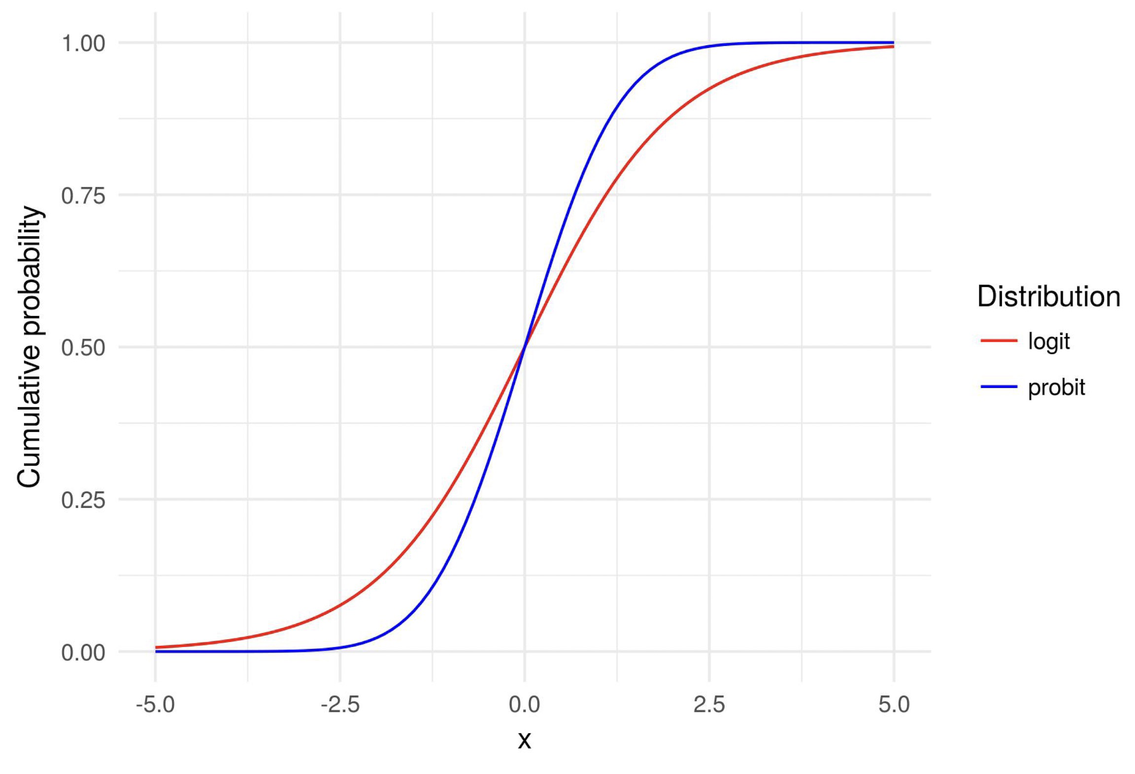
• Consider the following non-linear model:$$E(y \mid x)=P(y=1 \mid x)=G(\beta_0+\beta_1 x)$$where $G$ is a function mapping values to the range of 0 and 1 , to make sure $E(y \mid x)$ belongs to 0 and 1 .
• $G$ can have different functional forms. We consider two common ones:
  • logistic function （logit）
    • $$G(z)=\frac{\exp (z)}{1+\exp (z)}$$
  • standard normal CDF （probit）
    • $$G(z)=\Phi(z)$$
  • 

Properties of Logit and Probit

• y的这两种分布取决于残项e的分布
• Suppose random variable $e$ has a CDF:$$\operatorname{Pr}(e \leq z)=G(z)$$Here $G(z)$ can be either logit or probit.
• Let $y^*=\beta_0+\beta_1 x+e$, where $e$ is independent of $x$.
• $$\begin{aligned} P(y=1 \mid x) & =P(y^*>0 \mid x) =P(\beta_0+\beta_1 x+e>0 \mid x) \\ & =P(e>-\beta_0-\beta_1 x) =1-\operatorname{Pr}(e \leq-\beta_0-\beta_1 x) \\ & =1-G\left(-\beta_0-\beta_1 x\right)=G\left(\beta_0+\beta_1 x\right) .\end{aligned}$$

Partial effect of x on y

• the marginal effect of $x$ on the probability that $y=1$$$\frac{\partial p(x)}{\partial x_1}=g(\beta_0+\beta_1 x) \beta_1$$where $p(x)=P(y=1 \mid x), g(z) \equiv \frac{d G}{d z}(z)$.
  • 即对上面的式子求导
• When we have more than one independent variables:$$\frac{\partial p(x)}{\partial x_j}=g(\beta_0+\boldsymbol{x} \boldsymbol{\beta}) \beta_j$$where $\boldsymbol{x} \boldsymbol{\beta}=\beta_1 x_1+\ldots+\beta_k x_k$.

• So the ratio of the partial effect of $x_j$ and $x_k$ is $\frac{\beta_j}{\beta_k}$.
• 这种方法和OLS比的弱点在于这个偏导数的前项g取决于x
• 解决办法：
  1. 找特殊点，例如均值点。
     • Partial effect at the average:$$g(\hat{\beta_0}+\overline{\boldsymbol{x}}\hat{\beta_{\mathbf{1}}})=g(\hat{\beta_0}+\hat{\beta_1} \bar{x_1}+\hat{\beta_2} \bar{x_2}+\cdot+\hat{\beta_k} \bar{x_k})$$
  2. 求偏导的均值
     • Average marginal effect:$$[N^{-1} \sum_{i=1}^N g(\hat{\beta_0}+x_{i} \hat{\beta_1})] \hat{\beta_j}$$

Maximum Likelihood Estimation

• 估计：在样本中观察到某些值时y=1，另外一些值时y=0

• 使用最大似然估计找到 $\beta$ 使得这种成立的概率最大。

• 下面就是一个普通的求最大似然估计的过程，当作概统复习：

• Suppose we have a random sample of size $N$. Fix every $x$ and $\beta$, the probability that $y=1$ is:$$E(y \mid x)=P(y=1 \mid x)=G(\beta_0+\beta_1 x) \equiv G(\beta x) $$

• Then for any observation $y=0$ or $y=1$, its probability density function is:$$f(y \mid \beta x)=G(\beta x)^y[1-G(\beta x)]^{(1-y)}$$

• For a random sample, all observations are independent of each other. Then the probability that we observe the sample is: （ $i$ is the index for each observation）$$f({y_1, \ldots, y_N} \mid \beta x_i)=\prod_{i=1}^N[G(\beta x_i)]^{y_i}[1-G(\beta x_i)]^{(1-y_i)}$$

• Maximum likelihood estimation (MLE): maximize the probability that we observe the data:$$\max_{\boldsymbol{\beta}} f({y_1, \ldots, y_N} \mid \beta x_i)=\max_{\boldsymbol{\beta}} \prod_{i=1}^N[G(\beta x_i)]^{y_i}[1-G(\beta \boldsymbol{x}_{\boldsymbol{i}})]^{(1-y_i)}$$

• Take the natural logarithm and define:$$\ell_i(\beta)=\log ([G(\beta x_i)]^{y_i}[1-G(\beta x_i)]^{(1-y_i)})=y_i \log [G( x_i)]+(1-y_i) \log [1-G(\beta x_i)]$$
• Then we can equivalently write:$$\max_\beta \sum_{i=1}^N \ell_i(\beta)=\max_{\boldsymbol{\beta}} \sum_{y_i=1} \log [G(\beta x_{\boldsymbol{i}})]+\sum_{y_i=0} \log [1-G(\beta x_{\boldsymbol{i}})]$$
• MLE is consistent and asymptotically efficient.

MLE and OLS

• OLS用来估算线性模型
• MLE用来估计线性和非线性模型
• 当u服从正态分布时，MLE与OLS结果相同

Appendix

• $\color{red}{\text{Law of Iterated Expectation:}}$

  • $$\color{red}{E(y)=E[E(y|x)]}$$

• Summation operation

  • $$\sum_{i=1}^N(x_i-\bar{x})(y_i-\bar{y})=\sum_{i=1}^N(x_i-\bar{x})y_i=\sum_{i=1}^N(x_iy_i-\bar{x}\bar{y})$$

• Variance

  • $$\begin{aligned}
    \operatorname{Var}(X+a) & =\operatorname{Var}(X) \\
    \operatorname{Var}(a X) & =a^2 \operatorname{Var}(X) \\
    \operatorname{Var}(X) & =\operatorname{Cov}(X, X) \\
    \operatorname{Var}(a X+b Y) & =a^2 \operatorname{Var}(X)+b^2 \operatorname{Var}(Y)+2 a b \operatorname{Cov}(X, Y) \\
    \operatorname{Var}\left(\sum_{i=1}^N a_i X_i\right) & =\sum_{i, j=1}^N a_i a_j \operatorname{Cov}(X_i, X_j) \\
    & =\sum_{i=1}^N a_i^2 \operatorname{Var}(X_i)+\sum_{i \neq j} a_i a_j \operatorname{Cov}(X_i, X_j) \\
    & =\sum_{i=1}^N a_i^2 \operatorname{Var}(X_i)+2 \sum_{i=1}^N \sum_{j=i+1}^N a_i a_j \operatorname{Cov}(X_i, X_j) .
    \end{aligned}$$